eDNA data analysis
Background.
This workflow is designed to process sequence data from PCR products amplified from a number of environmental samples and sequenced as a single pool using Illumina compatible next generation sequencers. The primers should amplify products that can be sequenced in their entirety using short read sequencing (including the primer sequences) with Read1 and Read2 having an overlap greater than 10 base pairs. The expected structure of the primers from the 5' end should be 4 random nucleotides (NNNN), an index sequence such that the forward and reverse index combination is unique for each sample in the analysis and finally the amplicon specific primer sequence. Since the amplicons are expected to amplify sequences from a wide range of species, the amplicon specific sequences can contain degenerate positions. Once amplified, the products should be purified to remove primer dimers and any erroneously sized products. The individual amplicons should be quantified using an accurate method (i.e. NOT 260/280 UV absorption based methods) and pooled to form an equimolar pool of amplicons. This is then used to make a sequencing library using a Kit similar to the NEBNext Ultra genomic DNA kit. This library is then sequenced as is on the appropriate Illumina sequencer to produce the desired read depth.
The analysis pipeline is composed of a number of applications that run on either a standard Windows PC or a Linux server preferably a HPC operating the SGE queueing system.
Citation for description of method and primers
Novel Universal Primers for Metabarcoding eDNA Surveys of Marine Mammals and Other Marine Vertebrates
Elena Valsecchi, Jonas Bylemans, Simon J Goodman, Roberto Lombardi, Ian Carr, Laura Castellano, Andrea Galimberti, Paolo Galli
Environmental DNA 2 (4), 460-476
Abstract
Metabarcoding studies using environmental DNA (eDNA) and high‐throughput sequencing (HTS) are rapidly becoming an important tool for assessing and
monitoring marine biodiversity, detecting invasive species, and supporting basic ecological research. Several barcode loci targeting teleost fish and
elasmobranchs have previously been developed, but to date primer sets focusing on other marine megafauna, such as marine mammals, have received less
attention. Similarly, there have been few attempts to identify potentially “universal” barcode loci which may be informative across multiple marine
vertebrate orders. Here we describe the design and validation of two new sets of primers targeting hypervariable regions of the vertebrate mitochondrial
12S and 16S rRNA genes, which have conserved priming sites across virtually all cetaceans, pinnipeds, elasmobranchs, boney fish, sea turtles, and birds,
and amplify fragments with consistently high levels of taxonomically diagnostic sequence variation. “In silico” validation using the OBITOOLS software
showed our new barcode loci outperformed most existing vertebrate barcode loci for taxon detection and resolution. We also evaluated sequence diversity
and taxonomic resolution of the new barcode loci in 680 complete marine mammal mitochondrial genomes demonstrating that they are effective at resolving
amplicons for most taxa to the species level. Finally, we evaluated the performance of the primer sets with eDNA samples from aquarium communities with
known species composition. These new primers will potentially allow surveys of complete marine vertebrate communities in single HTS metabarcoding assessments,
simplifying workflows, reducing costs, and increasing accessibility to a wider range of investigators.
Sample de-multiplexing: Deconvolute
This application can be obtained from GitHub here (press the download button to obtain the application), while the source code etc is here.
A generic command to process the raw sequence data with Deconvolute is:
Deconvolute.exe $read1 $read2 $primers $indexes $output
Where:
- $read1 - the name with path of the read 1 data file as a gzip compressed fastq file
- $read2 - the name with path of the read 2 data file as a gzip compressed fastq file
- $primers - the name and path of a text file containing the sequences of the primers used to amplify the amplicons, one sequence per line and the sequence as its synthesised (the reverse primer is not reverse complemented)
- $indexes - the name with path of a text file containing the sequences of the indexes used to identify the primers. The files as the same format as the 'primers' file: one sequence per line and the indexes in the reverse primers are not reverse complemented. The indexes.txt files shows the format of a index file.
- $output - the path to a folder to save the output data in.
Initially, Deconvolute reads the first 100,000 reads in the read 1 and 2 files and produces a list of all the index combinations present in the files and creates an export *.fastq.gz file for each index pair that has more than 10 read pairs mapping to it. Once the export files have been made, the read pairs are checked to make sure they have different primers on each end, trimmed to remove low quality sequences and then combined to form a single sequence, which is then saved to the appropriate *.fastq.gz file.
Filtering and ordering sequences: SortFASTQ
This application can be obtained here. (press the download button to obtain the application), while the source code etc is here.
A generic command to process the data files from Deconvolute with SortFastq is:
SortFastQ.exe $fastqFile $output A
Where:
- $fastqFile - the name with path of the fastq file to process
- A or Q - the presence of A or Q sets the the format of the exported file Q = fastq and A = fasta.
This application processes a single fastq file exported by Deconvolute and orders the reads by sequence name which Deconvolutes has set to the random NNNN sequence in each primer and the target specific sequences that amplified the PCR product. Sequences with duplicate names are filter such that only one is retained and saved to the export file.
Counting reads for each amplicon sequence and generating a list of unique amplicon sequences: Aggregator
This application can be obtained here. (press the download button to obtain the application), while the source code etc is here.
A generic command to process a folder of fasta files exported by SortFastq using Aggregator is:
Aggregator.exe $folder $size
Where:
- $folder - the path to the folder of fasta files exported by SortFastQ that will be included in the analysis
- $size - the typical size of the expected amplicon
This application in reads each of the fasta file in the folder and counts the number of times each amplicon sequence is found in each data file. This data is then exported as a tab delimited text file linking each amplicon sequence to the number of times it is found in each sample file. This data is linked to the amplicon sequence which is also exported to a fasta file that contains a list of unique amplicon sequences present in the data set.
Identifying the species of origin of each amplicon sequence.
This process is performed using a set of bash and python scripts as well as a local installation of the blastn application.
Prepairing the amplicon sequence file produced by Aggregator
Since the list of unique amplicon sequences can be very large the list is exported to a series of fasta files each containing 5,000 sequences.
A bash script to perform this task can be found here.
A generic command to run this script is:
bash b_CutUpFasta.sh $file
where:
- $file - the name with path of the file to split up.
This script creates a folder in the same folder as the fasta file, with the same name as the fasta file except the *.fa is charged to *_fa. Each set of 5,000 sequence are then saved to this folder as a series of fasta files.
Identifying the origin of each amplicon sequence using blastn
The blastn application along with the appropriate database can be downloaded from the NCBI website.
A qsub bash script for use with the SGE queuing system found on many HPC systems can be found here.
A generic command to run this script (as one unbroken line) via qsub is:
qsub -t 1-n -v folder=<folder>,blastdb=<blastn database> qs_BlastnSearchLoop_eDNA_10Hits.sh
Where:
- n the number of fasta files generated by b_CutUpFasta.sh
- <folder> the folder with path of the directory that contains the fasta files
- <blastndatabase> the name and path to the blastn database to be searched by blastn
Processing the list of unique amplicon files with blastn is a slow process, but by breaking the list up in to a series of smaller data sets which are then processed in parallel using a high performance computer cluster allows this task to be processed in less than a day when the non-redundant genbank DNA data base is screened by the amplicon sequences. The amount of resources required depends on the size of the database screened. The example script requests 5 cores with a total of 75 Gbytes of ram for 48 hours, which will sufficient for the Genbank nr database, which is currently the largest database. This script creates a subfolder in which the results of the screening is saved as a series of xml files, which each contains the top ten hits for each of 50 amplicon sequences. If the script doesn't complete before all the sequences have been blasted, remove the *.txt files in the subfolders and requeue the script whih should restart from the last successfull search.
Aggregating the results of the blastn analysis to a single file.
A python script that aggregates the results of the blastn analysis can be found here.
A generic command to run this script is:
python p_Get_Blast_Data_From_Folder_of_Folders_with_seq.py $folder
Where:
- $folder - the folder name with path of the folder in result folders are located (i.e. this is the same folder used in the qsub command).
This script creates a tab delimited text file called 'Alignment_Details.txt' which contains data from the blastn results linking each amplicon sequence to a maximum of ten blast hits, giving the hit's description and accession ID as well as parameters defining the quality of the alignment.
Adding taxonomic data to sequence: AddTaxonomyToCountsSetGroup
This application can be obtained here (press the download button to obtain the application), while the source code etc is here
AddTaxonomyToCountsSetGroup is a windows base application with a user interface that connects to a ITIS database run using either Microsoft's SQL server or a SQLExpress instance.
User guide
The taxonomic data is retrieved form a SQL server or SQLExpress instance hosting a copy of the ITIS database (ITIS Downloads). When AddTaxonomyToCountsSetGroup starts it shows the window (Figure 1) which allows the user to enter a connection string and gives two generic strings for SQLExpress and a SQL server instances highlighted in bold. Clicking on the bold text will copy it to the text box. This string requires the name of the server, which if the server is on the local machine is the computer's name and is already added to the string. If the SQL server is on another machine, this will have to be manually added. If necessary a username and password for the database will need to be entered. More information on connection strings can be found here: Microsoft SqlClient Data Provider for SQL Server Connection Strings - ConnectionStrings.com.
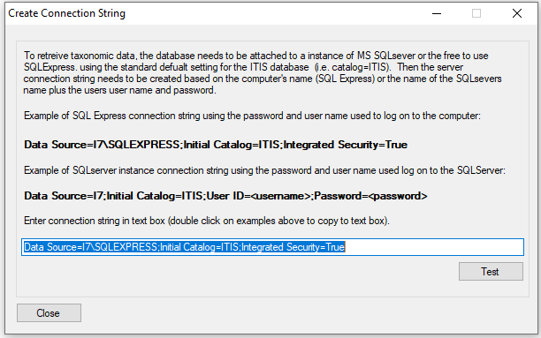
Figure 1: connecting to the ITIS database
Once the connection string is entered, press the button and a dialog box will appear stating if a connection could be made.
If successful, press the button and the main user interface will appear (Figure 2). Using this window, enter the data aggregated
by the p_Get_Blast_Data_From_Folder_of_Folders_with_seq.py python script by pressing the button
and the Read count data generated by Aggregator by pressing the button. Once the read count
and aggregated blast data result files have been selected, the data is processed by pressing the button. This process is achieved
in four main steps with the analysis status show in the panel in the lower half of the window.
Step 1: Creating a list of species names from data base. This step collects all the names of each species with associated data from the ITIS database.
Step 2: Getting Taxonomic data from the ITIS database: This step collects all taxonomic features with associated data needed to create a phylogenetic string
for each species.
Step 3: Reading the blast data file: The blast results data file contains up to 10 hits for each sequence exported by Aggregator, in
this step, each result is read in turn until the species name extracted from the accession's description can be linked to species or family name collected from
the ITIS database. Once linked the species name is linked to its phylogenetic data.
Step 4: Reading the counts file and saving results to file: The read count data is read with the data for each sequence linked to the
phylogenetic data created in step 3. This data is then save to a file.
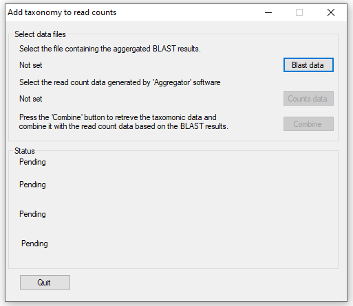
Figure 2: AddTaxonomyToCountsSetGrou main interface
Combining amplicon sequences based on taxonomy and filtering on read count: FilterrRNAData
This application can be obtained here (press the download button to obtain the application), while the source code etc is here.
FilterrRNAData is a windows base application with a user interface. The program filters the data exported by AddTaxonomyToCountsSetGroup based on sample name, amplicon alignment length and homology to the Blastn hit sequence used to annotate the sequence.
User guide
FilterrRNAData consists of a single user interface that allows the data file exported by AddTaxonomyToCountsSetGroup to be filtered based on the Blast alignment data and then aggregated based on each sequence's phylogenetic annotation.
Figure 3 shows the user interface displayed when the application is started. The panel allows
the parameters for filtering the data to be adjusted.
allows the minimum and maximum amplicon length to be set: amplicon sequences outside this range
are excluded.
allows the sequences to be filtered based on the alignment generated by Blastn. The default
value is 98%: such that sequences are only retained if 98% of the amplicon sequence is the same as the hit sequences identified by Blast. This value
can be set from 80% to 100%.
While homology at 80% is very likely to include an excess of incorrectly annotated sequences, a cut-off of 100% is likely to exclude many sequences
due to PCR and sequencing errors as well as sequences not present in the database, but which do have sequences from closely related species. Values
between 95% and 98% may be more appropriate.
sets the taxonomic level at which the read data is combined at. For instance, read count data
can be combined at the level of the 'Species' or 'Family' name, such that read counts linked to the same 'Species' name or 'Family' name are combine
to a single data point The phylogenetic data from ITIS contains 31 levels as shown in table 1. Not all species contain an entry for all of the levels,
consequently missing annotation is replaced by the previous enty's name proceeding a '.'.
Once the import options have been selected the data file is selected and imported by pressing the button. Once the
data has been imported changing the import parameters will not affect the analysis. As the data is imported, the status of the imported data is shown
in the panel. This gives the number of lines read in the imported file followed by the number of unique UTOs
that have been stored. This value relates to the number of discrete entities that are exported, for instance if the level is set to aggregate sequences
based on the their 'Clade' name all sequences linked to seals will be included a single 'Pinnipedia' entity, while if its set to 'Family', sequences linked
to seals will be split amongst 'Enaliarctidae', 'Desmatophocidae', 'Odobenidae', 'Otariidae' and 'Phocidae' entries if present. The panel also shows the
number of lines excluded due to being the wrong size or having an alignment homology below the cut off. When the data has been read, the last line contains
the total number of counts linked to the sequences exported in the final dataset.
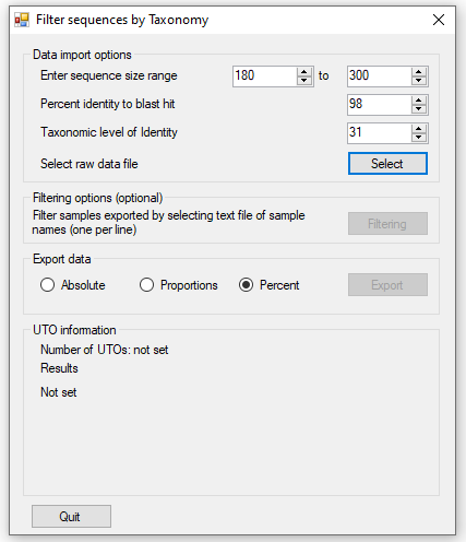
Figure 3: The User interface of FilterrRNAData.
| Name | Level |
| Kingdom | 1 |
| Subkingdom | 2 |
| Infrakingdom | 3 |
| Superdivision | 4 |
| Superphylum | 5 |
| Division | 6 |
| Phylum | 7 |
| Subdivision | 8 |
| Subphylum | 9 |
| Infradivision | 10 |
| Infraphylum | 11 |
| Parvdivision | 12 |
| Parvphylum | 13 |
| Superclass | 14 |
| Class | 15 |
| Subclass | 16 |
| Infraclass | 17 |
| Superorder | 18 |
| Order | 19 |
| Suborder | 20 |
| Infraorder | 21 |
| Section | 22 |
| Subsection | 23 |
| Superfamily | 24 |
| Family | 25 |
| Subfamily | 26 |
| Tribe | 27 |
| Subtribe | 28 |
| Genus | 29 |
| Subgenus | 30 |
| Species | 31 |
Table 1: Taxonomic level against phylogenetic feature as used by FilterrRNAData
Filtering and renaming sample based on their indexes:
The panel allows the samples to be renamed and filtered based on their indexes by importing a
tab-delimited text that contains the name of the sample and its index formatted as shown in table 2. The first line of the file consists of the column
headers (which aren't read by the program), while each subsequent line contains the samples name, a tab character and the indexes as given in the file
names exported by SortFASTQ.
If this file doesn't contain an index pairing, the data will not be exported by FilterrRNAData.
| Sample Code | <tab> | MV1 |
| ADG1a2.5 | <tab> | GGAGCGTC-GCGCTCTA |
| ADG1a5 | <tab> | AAGATACT-GCGCTCTA |
Table 2
Exporting the data
The panel allows the data to be save to a tab-delimited text wile with an *.xls file extension (as it is best viewed in Excel)
by pressing the button and then entering the name of the file to save the data too. The first column in the file contains the name of the
taxonomic grouping of the each row, while the subsequent rows, first include the read count data for each sample, followed by the taxonomic levels
from Kingdom to the user selected cut off level used to aggregate the sequences. The panel also contains three options that govern
how the read count data is exported.
exports the read counts as they are found in the data set with no adjustment for library size and differences in sizes of data between
the samples.
exports the read count data as the proportion exported reads in that sample that are linked to each taxonomic row in the file.
, like the option, this exports the data as a percentage of the reads linked to the specific
taxonomic grouping. (This is the value in the option x 100).
Downstream analysis
The exported file can then be used to create graphic representation of the data using a variety of software and R packages.
Original copies of the programs
While the main repository for the scripts and programs is on GitHub (https://github.com/msjimc/eDNA) the original versions can be found on this site here: